#9 - The Sheet

🔢 How to average the top 3 numbers in your data

Hey Friends,

It’s time for another edition of The Sheet - equipping you with time-saving tips each week!

Here’s what to expect in this week’s edition…

📋 Summary:

1. 💡 The Sheet Tip (Average your top 3 numbers)

2. 📚 What We're Reading: Entrepreneur Revolution by Daniel Priestley

---

=💡 The Sheet Tip (Average your top 3 numbers)

Today, we'll explore how to calculate the average of the top 3 numbers in a dataset.

Often, you may encounter situations where you want to focus on the highest values and analyse their average. Excel provides a powerful combination of functions to achieve this effortlessly. Instead of manually selecting and calculating the average, we can leverage the AVERAGE and LARGE functions together.

In Excel, the AVERAGE function calculates the average of a range. To narrow down our analysis to just the top 3 values, you can use the LARGE function.

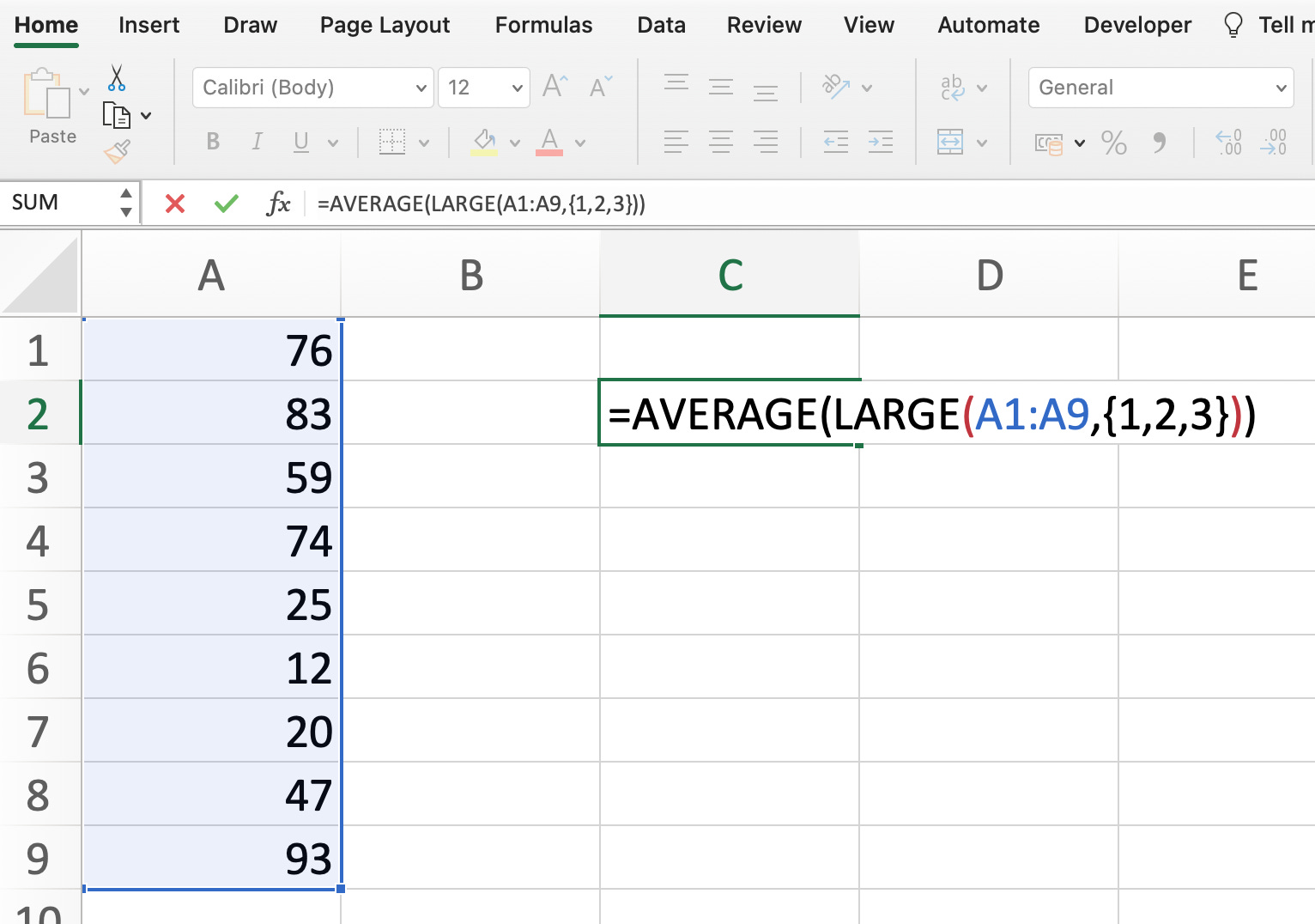
Here's the formula to get you started: =AVERAGE(LARGE(range, {1, 2, 3}))

In this formula, replace "range" with the actual range of your dataset. The array constant {1, 2, 3} signifies the positions of the top 3 values in the range. Excel will fetch those values and calculate their average. An example is provided below:

---

📚 What We're Reading: Entrepreneur Revolution: How to Develop your Entrepreneurial Mindset and Start a Business that Works - by Daniel Priestly

If you’ve ever wanted to unleash your inner Entrepreneur this is a must-read book. Priestly, a highly successful entrepreneur, describes how to break free from the ‘Industrial Revolution’ mindset. We found the book to be both inspiring and practical in terms of the initial steps you can take to start your entrepreneurial journey.

🖇️ If you’re interested in reading this book, we’d encourage you to check it out. Here’s a link to Amazon (Affiliate link).

---

Thanks for reading. If you found it useful, please hit that like button and share it with a friend or colleague.

See you next week.

The Functional Excel Team