#19 - The Sheet

3 shortcuts to turn your panic 😱 into calm 😎

Hey Friends,

Welcome back to the Sheet!

Have you tried out any new shortcuts from our shortcut guide? In case you missed it, you can download it using this link 😀.

If you haven’t tried any yet, here’s a common scenario you might face, where you can use 3 of the shortcuts in our guide….Buckle up…it’s a long one

---

=💡 The Sheet Tip (3 shortcuts to turn your panic 😱 into calm 😎 )

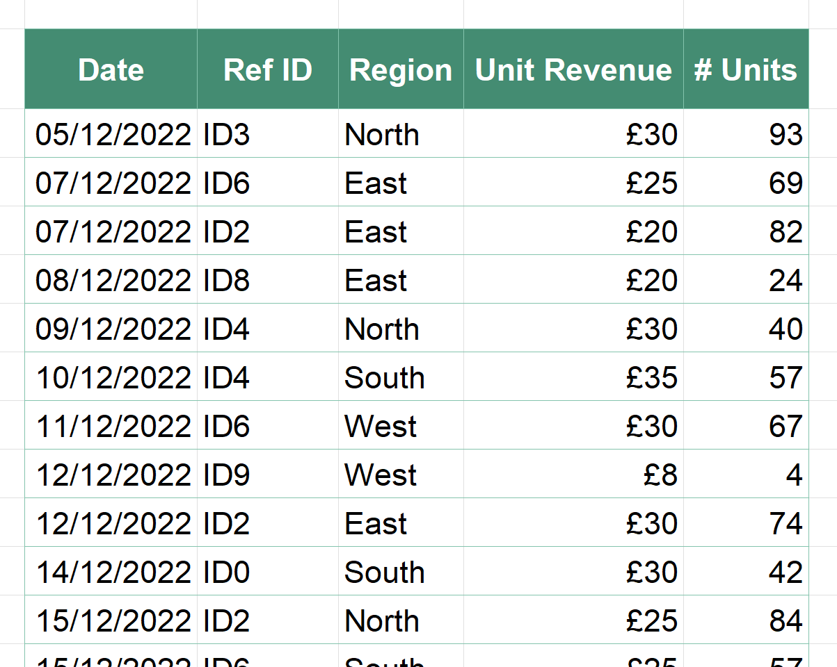
Picture this scenario. You’ve been given this data set 5 minutes ⏰ ahead of an important meeting and you quickly need to summarise the number of units sold by region…The panic sets in….We’ve all been there.

Next time you’re in this situation - sit back, relax, and use these 3 shortcuts…

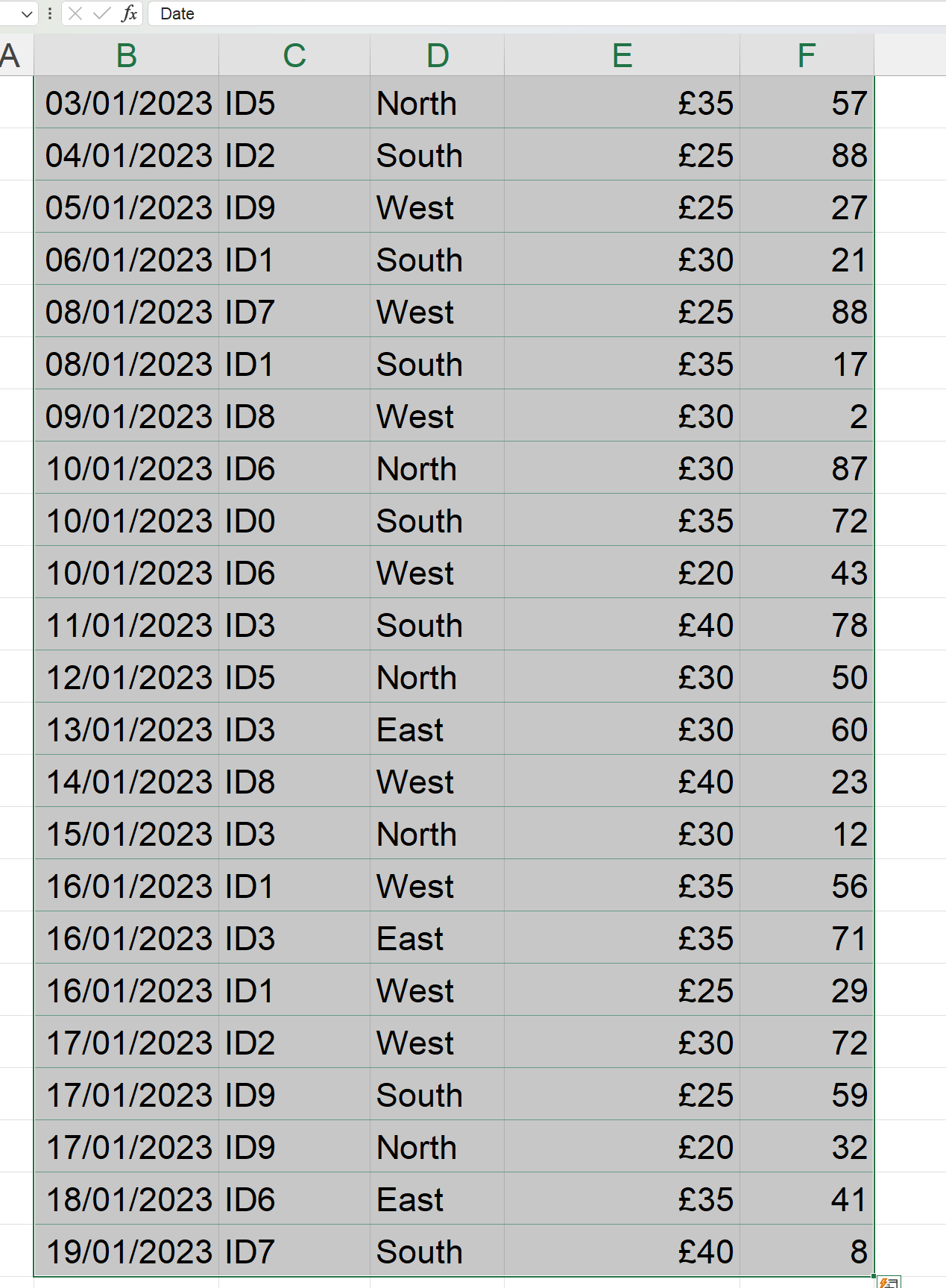
Step 1 - Select all the data [CTRL + A]

Click anywhere on the dataset and hit CRTL + A

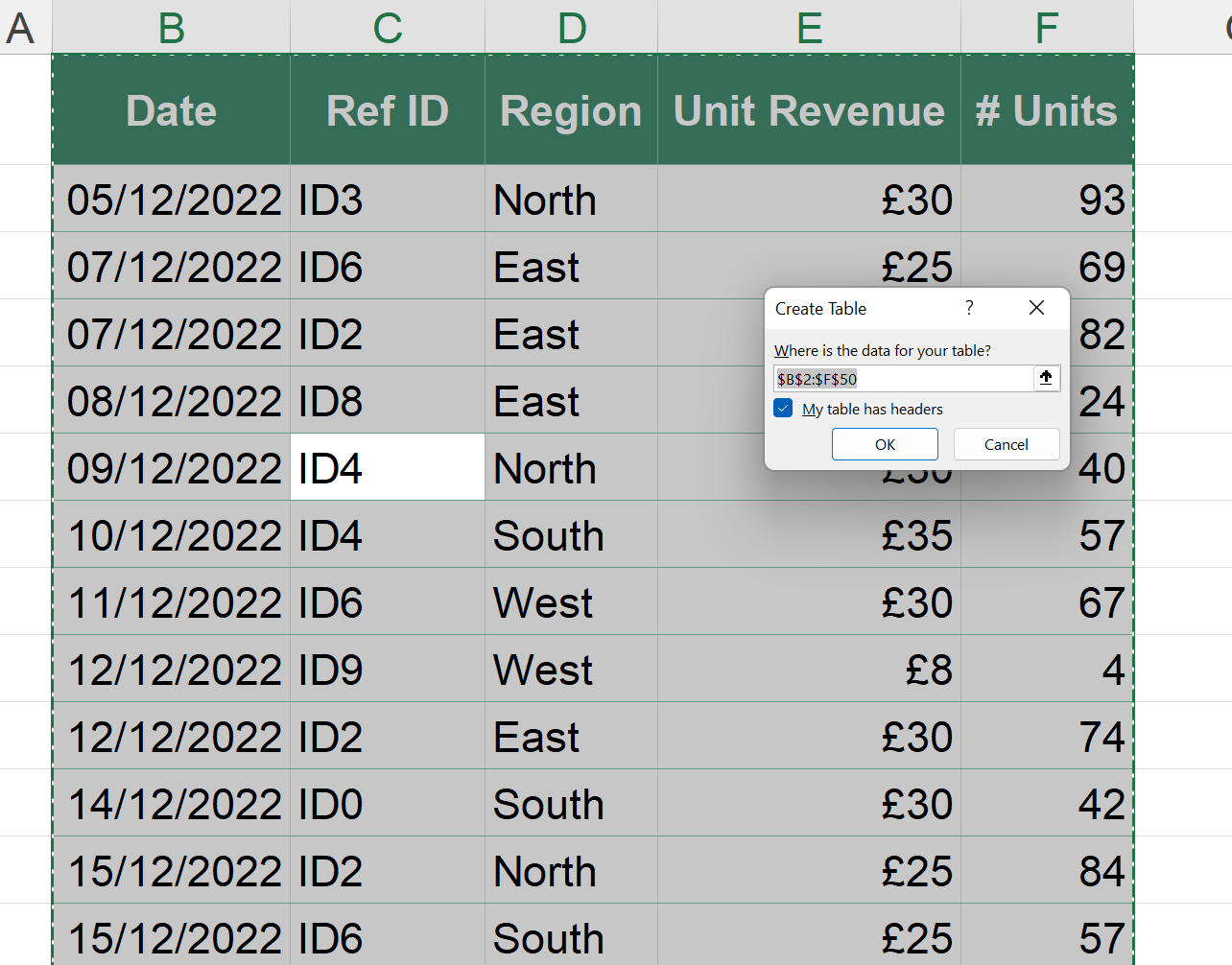
Step 2 - Turn your dataset into a table with [CTRL + T]

After selecting your data hit CTRL + T. Then, make sure the “My table has headers” dialogue box is ticked and press ‘OK’

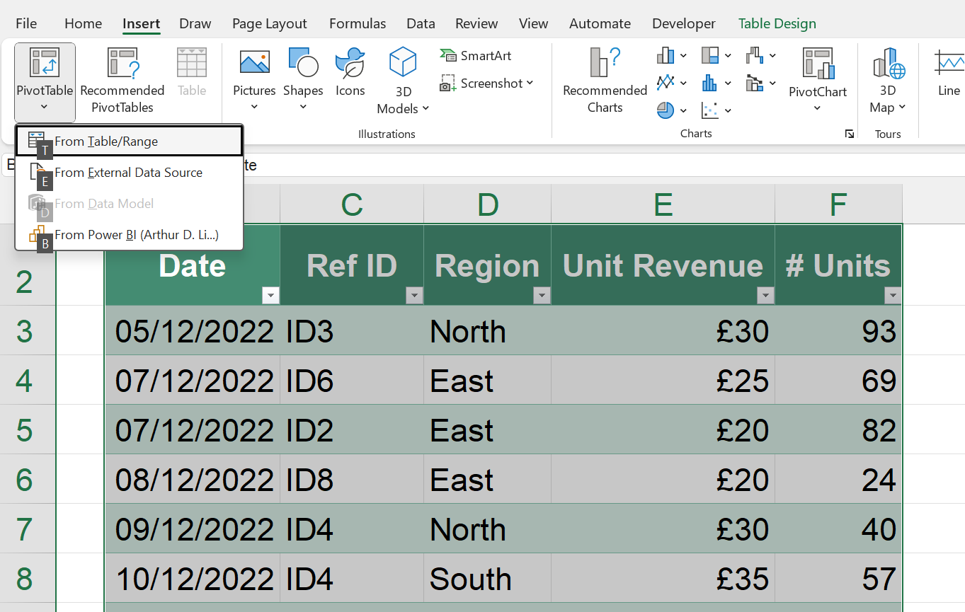
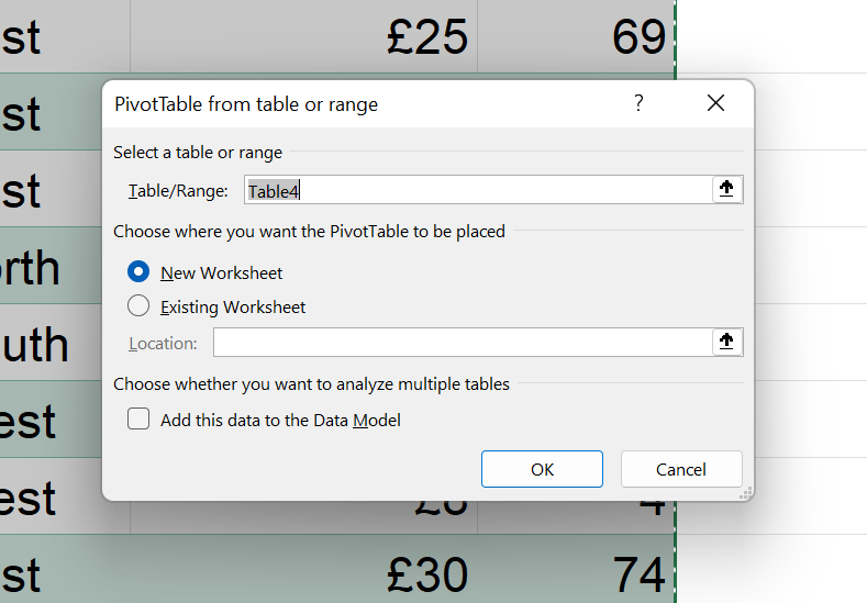
Step 3 - Create a Pivot Table [ALT + N, V]

Now that you have a table, hit the following keys Alt ➡️N➡️V➡️T (For a table)

Choose whether to add your pivot table to a new or existing worksheet and hit ‘OK’

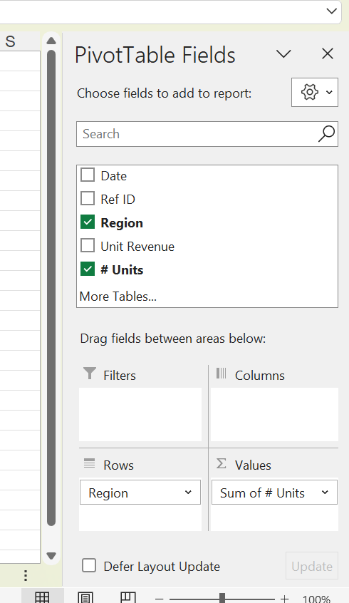
Step 3 - Tick some boxes

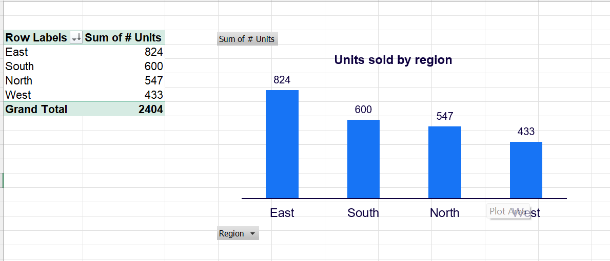
To populate your pivot table tick ‘Region’ and ‘# Units’ (It will automatically put ‘Region’ into Rows and ‘Sum of # Units’ into Values)

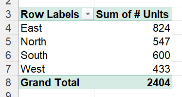
And there you have it…

Sneaky bonus content ⬇️

If you want to score some bonus points with your boss try these two extra steps:

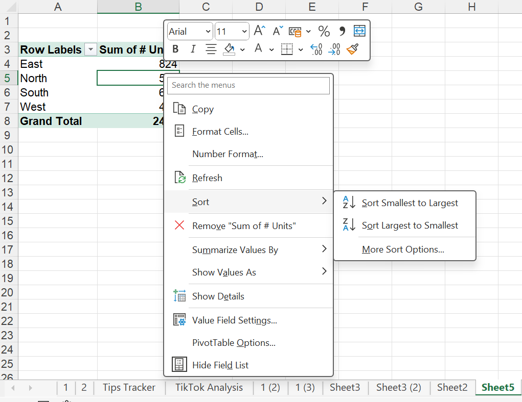
1. Right-click on 547 and go to ‘Sort’ then ‘Sort Largest to Smallest’

   

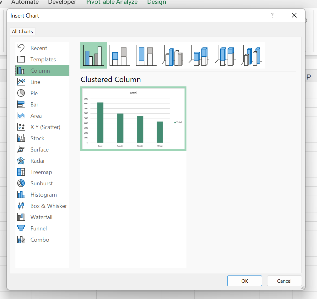
2. Go to Insert ➡️ Pivot Chart ➡️ Pivot Chart

   

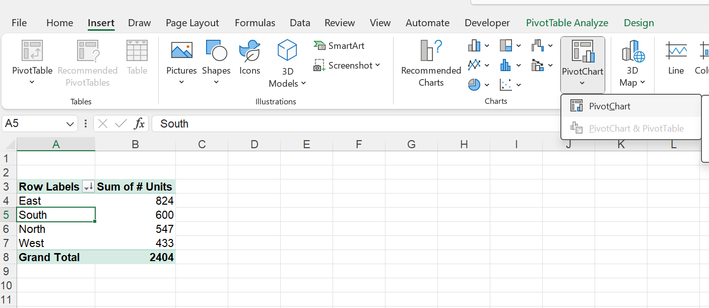
   Choose ‘Column’ and click ‘OK’

   

   …Who’s more impressed? You or your boss?

   

---

That’s it for this week.

See you soon!

The Functional Excel Team